INTRODUCTION
In 2016, Cyclistic launched a successful bike-share offering. Since then, the program has grown to a fleet of 5,824 bicycles that are geotracked and locked into a network of 692 stations across Chicago. The bikes can be unlocked from one station and returned to any other station in the system anytime.
Cyclistic categorized the riders as Casual who purchased single-ride or full-day passes and Members who purchased annual memberships.
Cyclistic’s marketing strategy relied heavily on building general awareness and appealing to broad consumer segments. Marketing team created flexibility on pricing plans like single-ride passes, full-day passes, and annual memberships. But there is no effort for an upselling plan to convert the casual riders into members.
Cyclistic’s finance analysts have concluded that annual members are much more profitable than casual riders.
Ms. Moreno, Director of Marketing Team, has a clear goal: Design marketing strategies aimed at converting casual riders into annual members. As a Junior Analyst in the Marketing Team, I was assigned to answer: How do annual members and casual riders use Cyclistic bikes differently?
BUSINESS TASK
Identify, analyze, and assess the bike usage trends and patterns of casual riders/members for the Cyclistic future marketing program.
DATA SOURCES
Internal data of Cyclistics was used in this case study under Motivate International Inc, under license. It is the original data from the source. A 12-month (November 2021 to October 2022) historical dataset was downloaded and stored in Google Drive and organized in a YYYYMM_CompanyName manner. To avoid sampling bias we will use the dataset that will represent the population and anonymization was used to implement data privacy.
Reliable — it is first-party data. It is owned by Cyclistic.
Original — Dataset is straight from the source. Although already anonymized the other data is still intact.
Comprehensive — There is some nulls but the importance of it can be checked in “Process” stage.
Current — Data is up to date and has the current information of the cyclers’ usage.
Cited — The City of Chicago owns all right, title, and interest in the Data. Thus, this is a reliable data source.
Since the finance analysts already concluded the annual memberships are much more profitable, anonymized data provided will help to focus on the main task which is to define the different usage of the bike renters.
CLEANING OR MANIPULATION OF DATA
Since the data exceeds the allowable complimentary BigQuery sandbox, I loaded the dataset in pgAdmin4 to use SQL. Tableau Public was used to create an interactive visualization or a dashboard and for an easier way to check the relations between columns, I used Anaconda.
STEP 1: Creating a table named bike.
Since all of our downloaded files have similar features, it will be logical to create only one table. Using this kind command, you can easily manipulate the features into correct data types.
CREATE TABLE IF NOT EXISTS public.bike
(
    ride_id character varying COLLATE pg_catalog."default" NOT NULL,
    rideable_type character varying COLLATE pg_catalog."default",
    started_at timestamp without time zone,
    ended_at timestamp without time zone,
    start_station_name character varying COLLATE pg_catalog."default",
    start_station_id character varying COLLATE pg_catalog."default",
    end_station_name character varying COLLATE pg_catalog."default",
    end_station_id character varying COLLATE pg_catalog."default",
    start_lat numeric COLLATE pg_catalog."default",
    start_lng numeric COLLATE pg_catalog."default",
    end_lat numeric COLLATE pg_catalog."default",
    end_lng numeric COLLATE pg_catalog."default",
    member_casual character varying COLLATE pg_catalog."default",
    CONSTRAINT ride_pkey PRIMARY KEY (ride_id)
)
Ensure to use the correct data type for future data aggregation/manipulation and Tableau visualization.
STEP 2: Copying and merging data.
We will not use any JOIN or UNION command because we created only one table. Stacking the 12-month in the ride table created.
COPY bike
--FROM '/Users/wilmalapuz/Downloads/202111_Cyclistic.csv'
--FROM '/Users/wilmalapuz/Downloads/202112_Cyclistic.csv'
--FROM '/Users/wilmalapuz/Downloads/202201_Cyclistic.csv'
--FROM '/Users/wilmalapuz/Downloads/202202_Cyclistic.csv'
--FROM '/Users/wilmalapuz/Downloads/202203_Cyclistic.csv'
--FROM '/Users/wilmalapuz/Downloads/202204_Cyclistic.csv'
--FROM '/Users/wilmalapuz/Downloads/202205_Cyclistic.csv'
--FROM '/Users/wilmalapuz/Downloads/202206_Cyclistic.csv'
--FROM '/Users/wilmalapuz/Downloads/202207_Cyclistic.csv'
--FROM '/Users/wilmalapuz/Downloads/202208_Cyclistic.csv'
--FROM '/Users/wilmalapuz/Downloads/202209_Cyclistic.csv'
FROM '/Users/wilmalapuz/Downloads/202210_Cyclistic.csv'
DELIMITER ','
CSV Header;
STEP 3: Data Familiarization.
Schema of the table created.
SELECT *
FROM information_schema.columns
WHERE table_name = 'bike';
Checking the total rows of the table
SELECT COUNT(*)
FROM bike
Getting the head of the table
SELECT *
FROM bike
LIMIT 10
We need to know how many distinct observation per column
SELECT
    COUNT(DISTINCT ride_id) AS rideid
    ,COUNT(DISTINCT rideable_type) AS ridetype
    ,COUNT(DISTINCT started_at) AS startat
    ,COUNT(DISTINCT ended_at) AS endedat
    ,COUNT(DISTINCT start_station_name) AS startstation
    ,COUNT(DISTINCT start_station_id) AS startid
    ,COUNT(DISTINCT end_station_name) AS endtstation
    ,COUNT(DISTINCT end_station_id) AS endid
    ,COUNT(DISTINCT start_lat) AS startlat
    ,COUNT(DISTINCT start_lng) AS startlng
    ,COUNT(DISTINCT end_lat) AS endlat
    ,COUNT(DISTINCT end_lng) AS endlng
 ,COUNT(DISTINCT member_casual) AS membercasual
FROM bike
Since the count and count distinct of ride_id is the same, we will not use any delete duplicate function for this dataset.
How many nulls per column
select
  sum(case when ride_id is null then 1 else 0 end) rideid
  ,sum(case when rideable_type is null then 1 else 0 end) ridetype
  ,sum(case when started_at is null then 1 else 0 end) startat
  ,sum(case when ended_at is null then 1 else 0 end) endat
  ,sum(case when start_station_name is null then 1 else 0 end) startstation
  ,sum(case when start_station_id is null then 1 else 0 end) startid
  ,sum(case when end_station_name is null then 1 else 0 end) endtstation
  ,sum(case when end_station_id is null then 1 else 0 end) endid
  ,sum(case when start_lat is null then 1 else 0 end) startlat
  ,sum(case when start_lng is null then 1 else 0 end) startlng
  ,sum(case when end_lat is null then 1 else 0 end) endlat
  ,sum(case when end_lng is null then 1 else 0 end) endlng
  ,sum(case when member_casual is null then 1 else 0 end) membercasual
from bike
We will go on to the next dataset feature which is the rideable_type.
SELECT rideable_type, COUNT(rideable_type)
FROM bike
GROUP BY rideable_type
ORDER BY COUNT(rideable_type) ASC
There are 3 classes of types in this data; docked, classic and electric.
SELECT started_at, ended_at
FROM bike
ORDER BY started_at ASC
STEP 4: Adding/Dropping columns for data analysis.
Going back to our business question, which is to analyze the bike usage of members and casual riders, we will now list all the underlying queries that we can formulate to answer the business task.
-What is the popular start time of the cyclers?
-What is the average cycling time?
-What is the busiest and slowest day/month?
-What is the average distance per cycle?
-Where is the most active station/dormant station?
By those questions above, we will need to drop the end_station_names and station_id column which consists of almost 1 million NULLS per column. We will add columns like starttime (extracted from started_at), cycletime (elapsed time between ended_at and started_at), month/day/year (convert the timestamp to their designated month/day/year), and distance traveled (using point command).
SELECT ride_id, rideable_type, started_at, ended_at, start_station_name AS station_name, start_lat, start_lng, end_lat, end_lng, member_casual
    ,started_at::time AS starttime
    ,extract
     (
             epoch from ((ended_at - started_at)/60)::interval
        )
         as cycletime
 ,TO_CHAR(started_at, 'fmDay') AS "day"
 ,TO_CHAR(started_at, 'fmMonth') AS "month"
    ,TO_CHAR(started_at, 'YYYY') AS "year"
 ,((point(start_lng, start_lat) <@> point(end_lng, end_lat)) * 1.609)as distance
FROM bike
WHERE start_lat != end_lat AND start_lng != end_lng
We will not stop there, we want to clean it further by using the ORDER BY command on our newly added column. We found out that there are negative cycle times and less than 5 meters cycling distance in some recorded rides. We will exclude those using the command below:
SELECT *
from (SELECT ride_id, rideable_type, started_at, ended_at, start_station_name AS station_name, start_lat, start_lng, end_lat, end_lng, member_casual
    ,started_at::time AS starttime
    ,extract
     (
             epoch from ((ended_at - started_at)/60)::interval
        )
         as cycletime
 ,TO_CHAR(started_at, 'fmDay') AS "day"
 ,TO_CHAR(started_at, 'fmMonth') AS "month"
    ,TO_CHAR(started_at, 'YYYY') AS "year"
 ,((point(start_lng, start_lat) <@> point(end_lng, end_lat)) * 1.609)as distance
FROM bike
WHERE start_lat != end_lat AND start_lng != end_lng) as Q
WHERE Q.cycletime >2 AND Q.distance > 0.005
With that, we only now have 5,091,767 rows for us to upload in Tableau.
ANALYSIS SUMMARY
We will use Tableau to answer our questions that will help us to derive our recommendations.
 |
| Google Capstone Case Study by Wilma Lapuz |
What is the median Travel Time?
 |
| Casual Riders strolled more than the Members |
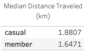
What is the median distance per bike rented?
 |
| Casual Riders had covers more distance than the Members |
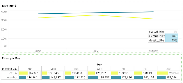
What is the busiest and slowest day/month?
 |
| Casual Riders: Busiest July | Slowest January | Busiest Saturday | Slowest Tuesday WHILE Member Busiest August | Slowest January | Busiest Thursday | Slowest Sunday |
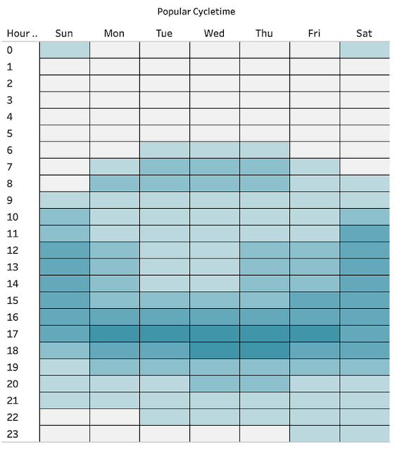
What is the popular start time of the cyclers?
 |
| Casual - Saturdays around 1500Hrs Members - Tuesdays by 1700Hrs |
Where is the most active station/dormant station?
 |
| Most Active for Casual Riders: Streeter Dr & Grand Ave |
Is there a trend or patterns in renters usage?
 |
| Winter |
 |
| Spring |
 |
| Summer |
 |
| Autumn |
The Spring Season figure shows that there is a positive upward trend of renters at the end of season. Then there is a steady trend of bike rentals n the Summer season and negative down slope when the winter is nearing.
Classic bikes are opted to be rented in the Summer and Winter season too while electric bikes are the popular choice for Spring and Autumn season.
Is there a correlation?
To prove if there is correlation between number of rented bikes and season, I downloaded the average temperature history and loaded it in Anaconda.
import pandas as pd
tempcalc = pd.read_csv('temp_calc.csv')
tempcalc.corr() |
| Correlation |
A correlation coefficient of is too far from 1, meaning there is no linear relationship.
KEY FINDINGS
- Members rented 60% of the total rides.
- 53% of Casual Riders prefer electric bikes while 54% of Members chose classic bikes.
- Casual Riders travel longer and farther than the Member.
- The usual starting station of Members are from the community area while Casual Riders are from Chicago’s Bay Area.
- Season affects the bike rentals.
RECOMMENDATIONS
Since demographics of bike users were anonymized, the recommendations will only evolve in the three variables: kind of bike rented, stations and time.
Create an Exclusive Membership Reward Points System:
- Friday, Saturday, and Sunday by 3PM is the peak period for casual riders, thus an exclusive membership reward program will offer their leisure rides extra reward points while using bikes on the said peak periods from those popular stations.
- Casual riders also be offered a discounted rate per minute for the electric bike for the first three months.
- For members, they will receive reward points for every rider that will purchase an annual membership using their invite code.
Voucher Codes
- Casual riders may increase their annual membership discount based on their past bike rentals to and from the popular stations.
- Voucher codes for annual membership can be offered at the start of Spring Season in preparation for the upcoming peak rental season.
Exclusive for Health Enthusiast Members
- Since casual riders were fond of renting an electric bike, Cyclistic may promote the use of classic bike and entice them by challenge badges that can be shared in social media.
- Casual riders may have the option to save their cycled routes and to be featured on next popular/new discovered exploration routes in Cyclistic website.
- Promote an extended free cycling time for members and accompanying health benefits if they cycle on weekends’ off-peak times from 5AM — 9AM.
FOR FURTHER EXPLORATION
- Check the age brackets and financial capacity of casual riders and then create a focus group to discuss their takes on current membership strategy of Cyclistic.
REFERENCES
- DATA SOURCE: https://divvy-tripdata.s3.amazonaws.com/index.html
- DASHBOARD: WML CYCLISTIC CASE STUDY 2022
- PRESENTATION: UNDERSTANDING THE RIDE!
- LINKEDIN: WILMA LAPUZ


